The stress–strain curve is one of the most common graphs you’ll meet in introductory materials science or mechanics of materials. Although its many labeled points and regions can seem daunting at first, both plotting and mastering stress versus strain are actually quite straightforward. In this article, we’ll explore the stress–strain curve in detail so you can understand it better.
But before we get started, let’s first review the answers to these questions:
1. Why define a material’s properties with stress–strain rather than force–displacement?
Force–displacement curves depend on a specimen’s size and shape—a thicker or longer sample requires more force (and undergoes a different displacement) even if it’s the same material. In other words, force and displacement are extrinsic properties tied to geometry.
2. What Is Stress?
When an external load F is applied to a continuous, deformable component in static equilibrium, the component deforms and develops internal forces F′ that exactly oppose the applied load to maintain equilibrium. Assuming that F is uniformly distributed over a cross-sectional area A , the internal resisting force per unit area is known as stress and can be expressed as:
Stress has units of pressure (Pa or N/m²) and represents the average internal force per unit area resisting deformation. This engineering stress formula assumes a uniform stress distribution; for large deformations or highly non-uniform loading, use true stress (based on the instantaneous area) or the full stress tensor for precise analysis.
3. What Is Strain?
Under an applied load, the material deforms. To compare deformation across specimens of different sizes and shapes, scientists introduce a non-dimensional measure called strain, which quantifies relative elongation.
For an element with original length L0 and change in length ΔL, the engineering strain is defined as:
Engineering strain is simple and accurate for small deformations (typically up to ~5 %). For large deformations, such as in metal forming or nonlinear FEA, you use true (logarithmic) strain, which accounts for the continuously changing length:
What Is the Stress-Strain Curve?
A stress-strain curve shows how a material behaves under load, which provides insights into the material’s strength, stiffness, ductility, and failure limits.
How is the Stress - Strain Curve Measured?
It is typically measured by a destructive uniaxial tensile test: a standardized “dog-bone” or straight-rod specimen is gripped in a Universal Testing Machine (UTM). The machine applies the load at a controlled constant rate until the specimen fails. During this process, the UTM’s load cell measures the tensile force F, while an extensometer (or video/DIC system) records axial deformation over the defined gauge length. Force vs. displacement—and hence engineering stress vs. engineering strain—is recorded continuously. Finally, you convert force to stress (σ=F/A0) and displacement to strain (ε=ΔL/L0), then plot σ on the vertical axis versus ε on the horizontal axis to generate the stress–strain curve.
Stages of a Stress-Strain Curve
Stress–strain curves for ductile materials consist of multiple sections that reflect how the material responds as stress increases. Curves for brittle materials, by contrast, are much simpler - typically a straight line up to fracture. In the following, we’ll focus on the stress–strain behavior of ductile materials.
There are three main stages and five key points on the curve:
Three Stages
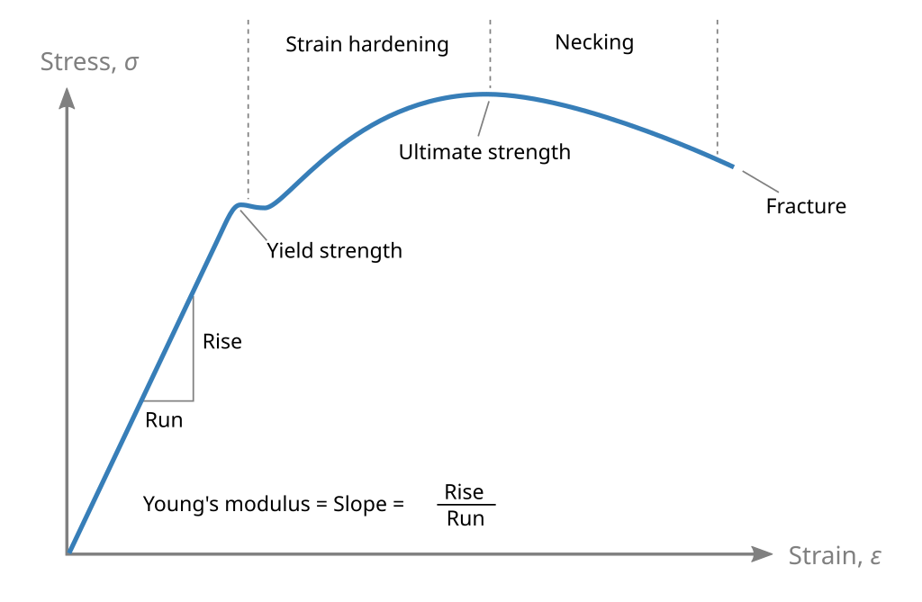
Elastic Deformation: In the initial portion of the curve, stress and strain are perfectly proportional, following Hooke’s law. Here the material behaves like a spring—remove the load and it returns to its original shape. The slope of this linear region is Young’s modulus, which quantifies the material’s stiffness.
Strain Hardening: After the yield point—and any brief stress drop or plateau in some steels—the material enters the strain-hardening stage. Plastic deformation continues uniformly along the gauge length, and the metal grows stronger as dislocations accumulate and interact, making further slip more difficult. Consequently, the stress required to keep deforming the specimen rises until it reaches the ultimate tensile strength.
Necking: Once the material reaches its ultimate tensile strength, uniform deformation ends and a “neck” forms in one region. From that point on, it takes less force to push further plastic flow in the neck, so the engineering stress (still using the original cross-sectional area) falls until the specimen finally fractures.
Five Key Points
Proportional Limit: The end of the linear portion on the stress-strain curve which Young’s modulus can be pulled from by calculating the slope.
Elastic Limit: The highest stress at which deformation is still fully recoverable. In metals, it nearly coincides with the proportional limit.
Yield Point (Yield Strength): The stress at which permanent deformation begins. It’s found by drawing a line parallel to the initial (elastic) portion of the curve but offset by 0.2% strain; the intersection of that line with the stress–strain curve defines the yield strength.
Ultimate Tensile Strength:The peak engineering stress on the curve. Beyond this, necking begins. (Note: true stress continues to rise until fracture.)
Fracture (Breaking) Point: The end of the curve, where the material finally breaks.
Other Material Properties from the Stress–Strain Curve
Modulus of Resilience: The area under the elastic portion of the stress–strain curve, representing the energy per unit volume a material can absorb and release without permanent deformation. It’s a key parameter for designing springs, crash-worthy structures, and any component that must store and return energy elastically.
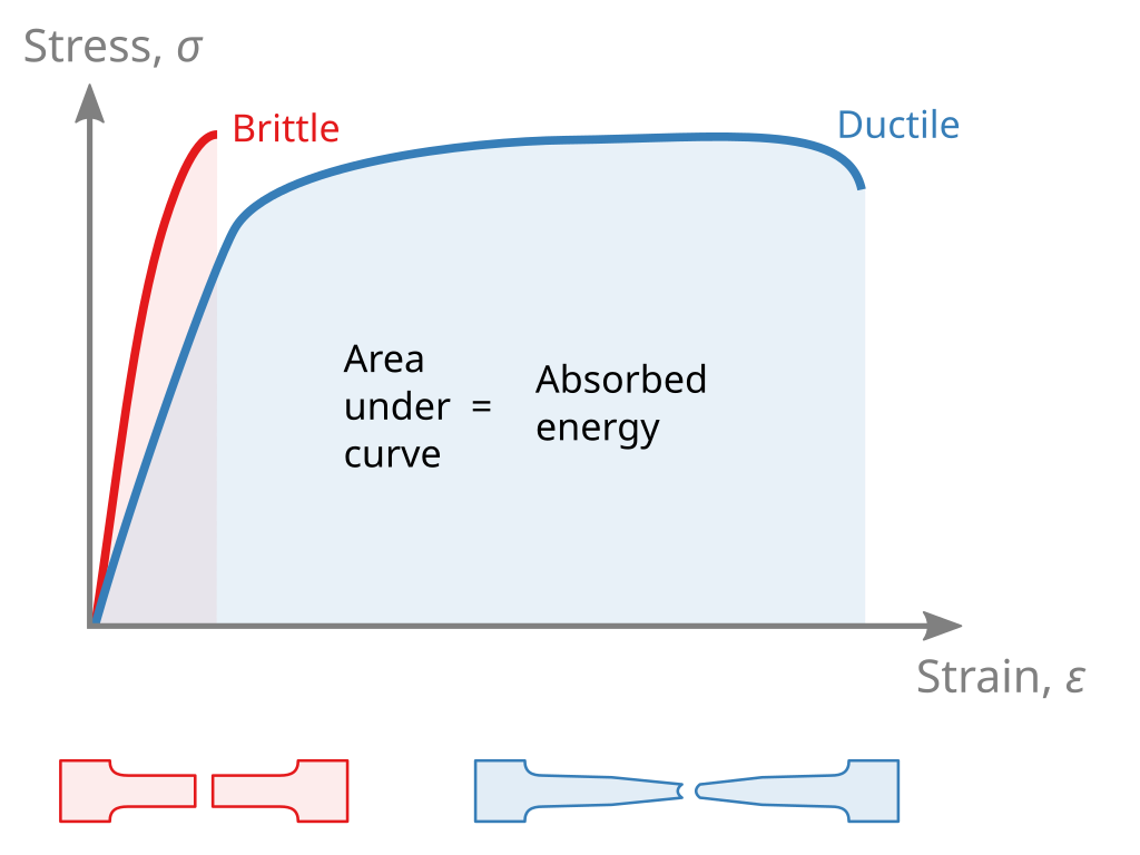
Toughness: The total area under the stress–strain curve, which quantifies the energy per unit volume a material can absorb before fracturing. Toughness guides the selection of materials for impact- and shock-resistant applications, such as automotive crash structures and ballistic armor.
Ductility: Measured by elongation at break (the percentage increase in gauge length at fracture) and reduction of area (the percentage decrease in cross-sectional area at the fracture), ductility measures how much a material can plastically deform before failing. High ductility is advantageous for forming operations, while low ductility indicates a higher risk of brittle fracture.
Work Hardening (Strain Hardening): After yield, true flow stress keeps rising with plastic strain in the uniform plastic region; this strengthening spreads strain more evenly, delays necking (greater uniform elongation), and improves metal forming (stamping, rolling, deep drawing) and FEA accuracy for springback and thinning.
Stress vs Strain Curves for Different Materials
Stress vs strain curves vary widely across material families. They can be broadly divided into two categories—ductile and brittle— as illustrated in the figure below.
Ductile materials, such as low-carbon steel, aluminum alloys, copper, and many thermoplastics, have a multi-stage stress–strain curve: an initial linear (elastic) region, a clear yield point, a strain-hardening (uniform plastic) region, necking, and finally fracture after substantial elongation. They can absorb large amounts of energy before failure.
Brittle materials, like cast iron, most ceramics, glass, and concrete, show almost purely linear elastic behavior up to fracture with virtually no plastic region, so their proportional limit, ultimate tensile strength, and fracture strength coincide.
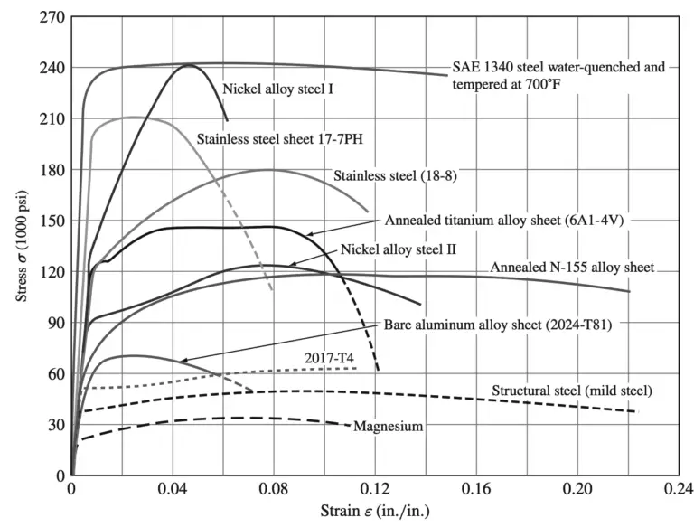
Note that the curves shown above represent only those specific material conditions. Actual stress–strain behavior can vary significantly with composition, heat treatment, microstructure, temperature, strain rate, and other test or processing parameters.
Engineering vs True Stress and Strain
Engineering and true stress–strain curves are the two most common ways to present tensile-test data.
Engineering Stress–Strain
In a standard tensile test, we assume the specimen’s cross-section stays at its original area A0. Engineering stress is therefore defined as:
and engineering strain as:
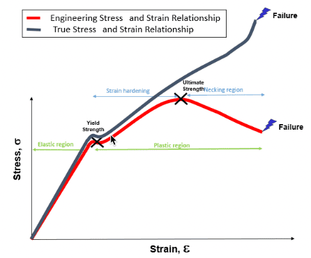
As you apply load, the curve rises linearly through the elastic region, then continues past the yield point into uniform plastic deformation, reaching its peak at the ultimate tensile strength—marking the end of uniform elongation. Beyond this peak, necking concentrates deformation into a narrowing section. Because engineering stress still divides by the original area A0, the plotted stress value drops even as the true stress (based on the shrinking area) continues to climb. Consequently, the engineering curve(shown in red in the figure)falls after UTS and trends downward until fracture.
True Stress–Strain
If you account for the instantaneous area Ai at each load step, you get true stress:
and true (logarithmic) strain:
During necking, the cross-sectional area decreases faster than the applied load falls so σt continues to rise beyond the engineering ultimate tensile strength. The true stress–strain curve therefore increases steadily up to fracture without dropping after its peak.
Engineering stress and strain are the standard data reported on material datasheets and used in design codes. They give quick access to familiar properties like yield strength, ultimate tensile strength, and elongation at break, making it easy to compare materials, set safety factors, and ensure consistent quality control across production batches.
True stress and strain are critical inputs for nonlinear finite-element analyses and constitutive models. By reflecting the real material response through large plastic strains and into necking, they enable accurate simulation of forming processes (e.g., stamping, forging, extrusion), precise springback predictions, and reliable forecasts of where and how a part will localize and ultimately fail.
Conclusion
The stress–strain curve is an indispensable tool that links material behavior to structural performance. It informs design by providing elastic modulus, yield strength, toughness, and ductility data used to size and qualify components. It also guides manufacturing by defining the stress–strain path needed to calculate forming forces, tooling geometry, and expected springback.
At Chiggo, we apply these material insights across a full suite of services, from CNC machining and 3D printing to sheet metal fabrication, and we’re pleased to provide free quotes and expert guidance for your next project.